Hukum Ohm Dan Rangkaian Seri – Paralel

Hukum Ohm menyatakan:

(http://abisabrina.wordpress.com)

“Besarnya kuat arus (I) yang melalui konduktor antara dua titik berbanding lurus dengan beda potensial atautegangan(V) di dua titik tersebut, dan berbanding terbalik dengan hambatan atau resistansi(R) di antara mereka

Dengan kata lain bahwa besar arus listrik (I) yang mengalir melalui sebuah hambatan (R) selalu berbanding lurus dengan beda potensial(V) yang diterapkan kepadanya.

Ilustrasi Hukum Ohm

Hukum Ohm dikemukakan oleh Georg Simon Ohm, fisikawan dari Jerman pada tahun 1825. Hukum Ohm kemudian dipublikasikan pada tahun 1827 melalui sebuah paper yang berjudul “The Galvanic Circuit Investigated Mathematically“.

Berikut ini contoh penerapan Hukum Ohm untuk menghidupkan lampu LED.

Penerapan Hukum Ohm

Menghitung Resistor Seri

Pada rangkaian beberapa resistor yang disusun seri, maka dapat diperoleh nilai resistor totalnya denganmenjumlah semua resistor yang disusun seri tersebut. Hal ini mengacu pada pengertian bahwa nilai kuat arus disemua titik pada rangkaian seri selalu sama.

Rangkaian Resistor Seri

Menghitung Resistor Paralel

Pada rangkaian beberapa resistor yang disusun secara paralel, perhitungan nilai resistor totalnya mengacu pada pengertian bahwa besar kuat arus yang masuk ke percabangan sama dengan besar kuat arus yang keluar dari percabangan (I in = I out). Dengan mengacu pada perhitungan Hukum Ohm maka dapat diperoleh rumus sebagai berikut.

Rangkaian Resistor Paralel

Menghitung Kapasitor Seri

Pada rangkaian kapasitor yang disusun seri maka nilai kapasitor totalnya diperoleh dengan perhitungan berikut.

Rangkaian Kapasitor Seri

Menghitung Kapasitor Paralel

Pada rangkaian beberapa kapasitor yang disusun secara paralel maka nilai kapasitor totalnya adalah penjumlahan dari semua nilai kapasitor yang disusun paralel tersebut.

Rangkaian Kapasitor Paralel

Cara Mudah Membaca Gelang Warna Resistor

Lazimnya gelang resistor terdapat 4 gelang kode yang umumnya digunakan untuk presisi rendah dengan toleransi 5%, 10% dan 20%. Gelang pertama dan kedua mewakili angka resistor. Gelang ketiga mengindikasi perkalian (multiplier) berapa ‘nol’ yang ditambahkan. Jika multiplier band adalah emas (gold) atau perak (silver) kemudian desimal digeser ke kiri satu atau dua (dibagi dengan 10 or 100). Gelang toleransi (tolerance band) deviasi dari nilai spesifik, biasanya terdapat jarak dari gelang lain.

Sebagai contoh, untuk resistor dengan nilai 560 ohm, 5% maka gelang warnanya adalah hijau, biru, coklat dan emas. Penjelasan: Hijau dan biru mewakili angka (56); sedangkan coklat adalah pengali (multiplier) (10) dan emas adalah toleransi (5%). Sedemikian sehingga nilainya 56*10 = 560.

Resitor dengan 5 gelang: Resistor dengan gelang seperti ini digunakan untuk rangkaian elektronika dengan presisi tinggi, resistor dengan presisi 2%, 1% atau bertoleransi lebih rendah. Cara membaca gelang mirip dengan sistem sebelumnya (4 gelang); hanya saja ada perbedaan nomor dari angka. Gelang pertama, kedua dan ketiga mewakili nilai angka, gelang ke empat adalah pengali (multiplier) dan gelang ke lima adalah toleransi.

Jika gelang ke tiga diubah ke warna merah, maka pengali (multiplier) akan menjadi 100, sehingga nilainya 56×100 = 5600 ohms = 5.6 k ohms. Jika gelang pengali (multiplier band) adalah emas atau perak, kemudian desimal poin akan digeser ke kiri satu atau dua tempat (dibagi dengan 10 atau 100). Sebagai contoh, sebuah resistor dengan gelang hijau, biru, perak dan emas mempunyai nilai 56*0.01 = 0.56.

Catatan: 20% resistors hanya mempunyai 3 gelang – artinya, gelang toleransi (gelang ke empat tanpa warna).

(source:http://coretancempluk.files.wordpress.com)

Standarisasi warna

Warna	Gelang ke-1	Gelang ke-2	Gelang ke-3 *	Pengali	Toleransi	Koefisien Suhu	Fail Rate
Hitam	0	0	0	×100
Coklat	1	1	1	×101	±1% (F)	100 ppm/K	1%
Merah	2	2	2	×102	±2% (G)	50 ppm/K	0.1%
Jingga	3	3	3	×103		15 ppm/K	0.01%
Kuning	4	4	4	×104		25 ppm/K	0.001%
Hijau	5	5	5	×105	±0.5% (D)
Biru	6	6	6	×106	±0.25%(C)
Ungu	7	7	7	×107	±0.1% (B)
Abu-abu	8	8	8	×108	±0.05% (A)
Putih	9	9	9	×109
Emas				×0.1	±5% (J)
Perak				×0.01	±10% (K)
Tanpa Warna					±20% (M)

* Gelang ke-3 hanya untuk 5-band resistors (source: http://pinginpintar.com/?p=236)

Tutorial Electronic Workbench 3

The oscilloscope

An oscilloscope is a far more powerful instrument than a bargraph indicator or even a voltmeter. It can show you the time dependence of the signals in your circuit. The EWB oscilloscope provides a fairly close approximation of a real one. It has two independent input channels, A and B, an input for an external trigger and a ground connection.

Figure 3. The EWB oscilloscope icon with its terminals.

To look at the output of your signal generator you can add anoscilloscope to the circuit you just made.

1. Drag the oscilloscope onto the circuit window, and double-click on it.The oscilloscope has four terminals, for two independent input channels, a trigger input and a ground connection. The input channels sense voltages with respect to ground! As long as there is at least one ground terminal attached to your circuit, it is not necessary to connect the oscilloscope ground. We will discuss the issue of how the oscilloscope is triggered in class. At this point, leave the triggering

on auto.

2. Connect channel A to the "+" output of the function generator, and

activate the circuit. You should now have a sine wave on your oscilloscope screen.

3. Make drastic changes in the signal amplitude and frequency, andadjust the sensitivity and time base settings such that you still maintain an easily interpretable picture of the wave form on the oscilloscope screen. It may be necessary to occasionally reactivate the simulation.

Figure 4. Using the oscilloscope to investigate the signals from the

function.

4. Change the offset on the function generator to a value of the order of

the amplitude. This adds a constant voltage to the signal. You will see

the trace on the oscilloscope move up (or down). You have two options

to move it back to center.

8

5. Change the "y position" such that the trace comes back on center.

This can always been done as long as the offset is not too large. (Most

oscilloscopes cannot produce an internal offset that is much larger

than the full scale display range.)

6. Change the "y-position" back to zero, and select "AC" as input

coupling mode. In this mode the DC component of the signal is

removed. The EWB oscilloscope is very good at this, but real

instruments have a difficulty distinguishing between DC and very

slowly oscillating signals. In practice, avoid the AC input mode for

signal frequencies less than 100 Hz.

To get a larger image of the oscilloscope, try the expand button. On the

expanded display you will find two vertical line cursors. By moving these

around you can measure time and amplitude of points on the displayed

traces.

Electronic WorkBench tutorial 2

Using the main instruments

EWB incorporates a number of instruments, such as an oscilloscope and a function generator. The following provides an introduction to these two instruments. To briefly investigate the function generator, build the circuit below.

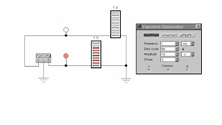
Figure 2. The function generator with bargraph displays.

The function generator

1. Drag the function generator onto the circuit window.

2. Double-click on the function generator. You can now change its settings, such as the wave form, the signal amplitude and the signal frequency.

3. The function generator has three terminals, "-", "common" and "+". Connect the common to a ground terminal.

4. Get two red probes from the Indicators toolbar. Wire them to the "+" and "-" terminals, and activate the circuit. You should now have two blinking red lights. To get a little bit more information we will attach a second kind of indicators.

5. Get two decoded bargraph displays form the indicator toolbar.

6. Wire one terminal of each of the bargraph indicators to ground, and the other terminals to the "+" and "-" terminals of the function generator.

7. Experiment with changing the wave form and frequency of the signal generator.

Electronic WorkBench tutorial

Introduction

Electronic WorkBench (EWB) is a simulation package for electronic circuits. It allows you to design and analyze circuits without using breadboards, real components or actual instruments. EWB's click-anddrag operations make editing a cir

cuit fast and easy. You can change parameters and circuit components on the fly, which make "what-if" analysis straight foreward.

This tutorial is intended as a quick introduction to E

WB's basic features. It first leads you through the fundamental steps of putting a circuit together and analyzing its function using the instruments. The final part of the tutorial consists of two exercises that try to illustrate the

power of EWB. It also tries to encourage you to apply the "what if" approach to circuit design. It will greatly help your understanding of electronics

if you use EWB in an interactive manner: Make change to the circuits you are working on, observe the effects that these changes have,

and try to understand them. EWB puts very little constraints on parameters so do not be too timid, don't just change things by 10%, try out what happens when you change them by a couple of orders in magnitude.

Directly printing EWB schematics and graphs does usually not produce satisfactory result, and leads to a tremendous waste of paper. It is bette

r to incorporate EWB results by copying them to the clipboard using the copy as bitmap command, and then pasting this into a something like a word document.

Directly printing EWB schematics and graphs does usually not produce satisfactory result, and leads to a tremendous waste of paper. It is better to incorporate EWB results by copying them to the clipboard using the copy as bitmap command, and then pasting this into a

something like a word document.

To open EWB click on its icon. Initially you will see an empty circuit window and two toolbars, the circuit toolbar with the common file ma

nagement, editing and graphics tools, and a Parts Bin toolbar from which you can select a wide range of circuit elements, and instruments. The following will guide you on your first attempt to simulate circuits.

Building and testing a circuit

In this part of the tutorial, you will build the simple DC voltage divider circuit shown below.

Figure 1. A resistive voltage divider

Step 1. Place the components on the circuit window

To build the circuit, you need a battery, two resistors and a ground connection. Assemble the components for the circuit.

1. Choose File/New to open a new circuit file.

2. Click in the Parts Bin toolbar. The basic toolbar should appear.

3. Drag two resistors from the toolbar to the circuit window.

To keep the Basics toolbar open, drag it onto the circuit window. Otherwise, it will close after you drag an item from it, and you will have to reopen it for every resistor.

4. Move to the Sources on the Parts Bin toolbar. Click on it and a toolbar containing the battery and ground should appear. Drag those onto the circuit window.

Step 2. Arranging the circuit elements

You can change the orientation of the circuit elements either by rotating them or flipping them over. To do this, select the circuit element and either click on the standard rotated/flip icons on the toolbar, or select the desired operation under Circuit. In this case you want to rotate both resistors.

1. Select both by either CTRL+click, or by dragging the mouse over them.

2. Choose your favorite way to rotate by 90 degrees.

Note that selected circuit elements are highlighted/changed color.

Step 3. Wire the components together

Most components have short lines pointing outwards, the terminals. To wire the components together you have to create wires between the components.

1. Move the pointer to the terminal on the top of the battery. When you are at the right position to make a connection, a black dot appears. Now drag the wire to the top of the upper resistor. Again a black dot appears, and the wire snaps into position.

2. Wire the rest of the components in a similar manner. You should end up with something like this:

Initially you wiring may not look very pretty. However, after making the connections, you can move wires and components around without breaking the connections.

Step 4. Set values for the components

Initially, each component comes up with a pre-set, default value, e.g., the battery voltage is set to 12 V. You can change all component values to suit your application.

1. Double-click on the component.

2. Select VALUE

3. Change its value.

4. Click OK.

Step 5. Save your circuit

Save your work frequently!

1. Select File/Save.

2. Proceed in the normal way for saving files.

Step 6. Attach the voltmeter

To measure voltages in your circuit you can use one or more voltmeters.

1. Drag a voltmeter from the indicator toolbar to the circuit window.

2. Drag wires from the voltmeter terminals to point in your circuit between which you want to measure the voltage.

3. Activate the circuit the circuit by clicking the power switch at the top right corner of the EWB window.

Step 7. Make changes and additions

You now have a very simple but functioning circuit. Take this opportunity to make some changes and additions.

1. Add an ammeter to the circuit to measure the current through the resistors.

2. Change the values of the resistors, and observe the change in the currents and voltages.

The ammeter can be connected by positioning it on top of the wire through which you want to measure the current. EWB will automatically make the right connections. If you are not sure that this is done correctly, drag the ammeter, the wires should move with it.

Note that the ground connection plays no particular role in this measurement. The voltmeter is not connected to a reference point. It functions very much like the hand-held multimeter in the lab. You can measure voltage differences between any pair of points in the circuit.